
In the first and second parts of this blog series, we discussed open datasets, and evaluation metrics for building footprint extraction. In this third and final part, we’re rounding out the series by reviewing model architectures for building footprint extraction including naive approaches, model improvement strategies, and three recent papers.
Naive Approaches
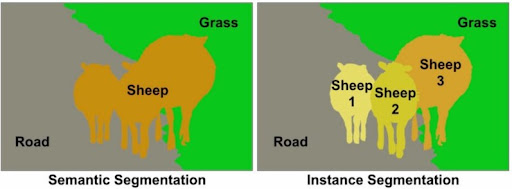
A popular, yet naive approach to building footprint extraction consists of three steps. First, a semantic segmentation model such as U-Net or DeepLab outputs a raster wherein each pixel indicates whether or not a building is present. Second, each connected component of building pixels is converted to a vectorized polygon using an off-the-shelf algorithm. Third, and optionally, a heuristic simplification algorithm such as Douglas-Peuker is applied to the polygons.
A problem with this approach is that semantic segmentation models are unable to delineate the boundaries between objects of the same class. This means that a single polygon will be drawn around a group of buildings that share walls, such as a block of rowhouses. To handle this case, the semantic segmentation model can be replaced with an instance segmentation model such as Mask R-CNN. This model generates a separate raster mask for each instance of a class that is detected.
Model Improvement Strategies
More recent and sophisticated approaches to building footprint extraction leverage two general strategies for improving deep learning models.
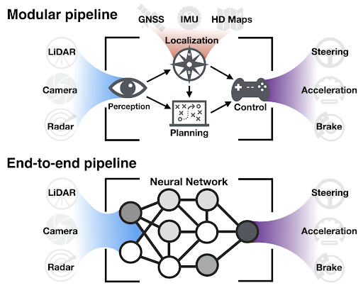
The first strategy is to train models “end-to-end” to directly produce the desired output from the input. For example, an end-to-end model for a self-driving car might predict a steering angle from an image. This is in contrast to a more traditional approach in which a model is trained to predict a map of the environment, which is then fed into a hard-coded motion planning algorithm to generate steering angles. By making the entire system trainable from data, it is possible to reduce errors that compound through the system, and optimize for the intended use case. This strategy has been applied to building footprint extraction by designing models that directly output polygons rather than rasters.
The second strategy is to incorporate a stronger inductive bias by utilizing a priori knowledge about the domain in the model and/or loss function. For example, a convolutional neural network (CNN) “bakes in” the notion of translation invariance. Translation invariance says that “a cat is a cat regardless of where it is in the image” by using the same weights to compute each pixel in a feature map. This strategy has been applied to building footprint extraction by designing models that are biased toward predicting building-like polygons that have low complexity and preserve corner angles.
Recent research on models for building footprint extraction
In the rest of this blog, we summarize three papers on models specially designed for building footprint extraction, and then conclude the blog series. These articles were all published recently, and exemplify one or both of the two model improvement strategies mentioned above. The models from the first two papers were used as the evaluation baselines for PolyWorld, the model in the third paper. Therefore, we present the evaluation of all these methods together at the end. Although these three models are architecturally diverse, this blog does not contain an exhaustive review of the literature. For this, we recommend consulting the related work sections of these papers.
Topological Map Extraction From Overhead Images
PolyMapper, published at ICCV 2019 by Li, Wegner, and Lucci [1], is a model that combines CNNs and RNNs to perform object detection, instance segmentation, and polygon extraction in an end-to-end fashion. It can be applied to both buildings and roads.
The first part of the model is similar to a Mask R-CNN, an instance segmentation model, which generates:
- a feature map for the image
- bounding boxes for each building
- and a crop of the feature map for each box.
Using the feature map for a bounding box, a fully convolutional model is used to generate a boundary mask and a vertex mask that is 1/8 the size of the input image. Each pixel in these masks stores the probability of being on a building boundary or vertex. The top K vertices are then selected and the one with the highest probability is selected as the first point in the polygon.
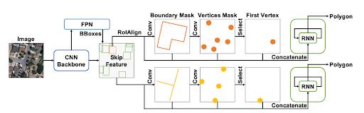
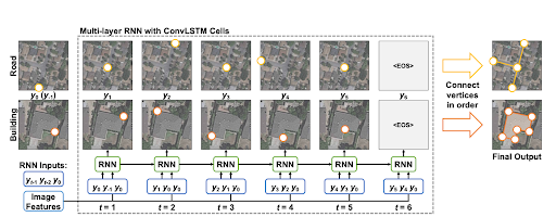
Next, an RNN with ConvLSTM cells is used to generate a sequence of vertices which are joined together to form a polygon. An RNN is used to generate a variable length sequence, which cannot be generated by a CNN. At each time step, the RNN takes the initial and the previous two points in the sequence, and the concatenation of the feature map, boundary mask, and vertex mask as input, and outputs a probability distribution over locations of the next vertex. When the last vertex matches the initial vertex, forming a closed polygon, the RNN outputs an end of sentence (EOS) token. The training loss combines losses over the bounding boxes, masks, and polygons.
PolyMapper can handle buildings that are touching, although it will not explicitly represent shared walls as such, and will duplicate them. It can also handle buildings with inner courtyards using polygons with holes, although it requires a modification that was not discussed here. The code for PolyMapper does not seem to be openly available.
Polygonal Building Segmentation by Frame Field Learning
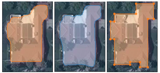
This paper was published at CVPR 2021 by Girard, Smirnov, Solomon, and Tarabalka [2]. The authors present a CNN that generates raster masks of polygon interiors and exteriors, and a frame field, an additional representation of contours and corners which facilitates downstream polygon extraction. Unlike the previous paper, this paper uses a polygon extraction process that is not learned end-to-end.
As can be seen below, a U-Net model is trained to output a boundary mask, and a frame field. The model is trained with a sum of various losses which can be broken into three categories: segmentation losses, frame field losses, and output coupling losses that enforce mutual consistency between the different outputs.
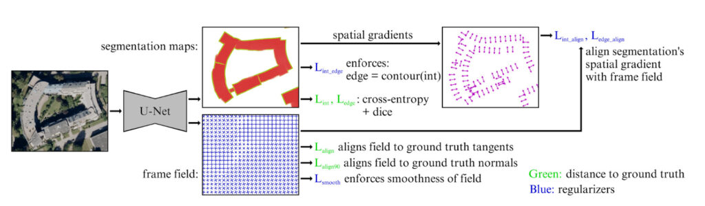
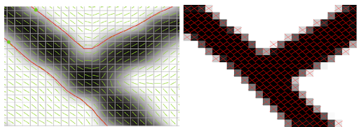
Tangent fields are a common representation for contours in an image, and consist of a 2D vector at each point that lies tangent to any contour nearby. They are good at modeling smooth curves, but struggle to represent sharp corners which are parameterized by two directions. Instead, frame fields (as instantiated in this paper) have a pair of vectors for each pixel. At corners, the vectors are aligned with tangents to the two constituent edges. Along edges, at least one vector is aligned to the edge. In the field of computer graphics, frame fields have been used to convert images of line drawings into vectorized graphics.
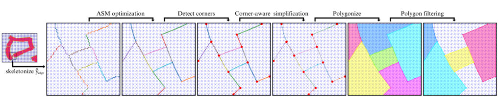
The output of the model is polygonized using a multi-step process which is depicted below. First, the boundary raster mask is thinned, and then converted to a set of contours using marching squares, a standard algorithm for extracting contours from rasters. Then, this graph is optimized using gradient descent to better align with the frame field and minimize complexity. Next, corners are detected and edges that connect corners are simplified. Finally, polygons are extracted and filtered to keep the ones that overlap with the polygon interior mask.
This method is able to handle buildings that are touching and buildings with courtyards by explicitly representing shared walls and generating polygons with holes. In addition, it runs about 10x faster than PolyMapper at inference time. The downside of this method is that the polygon extraction routine is complex and lacks the elegance of a model trained end-to-end. The source code is open source, but has a restrictive license that only permits its use for research.
PolyWorld: Polygonal Building Extraction with Graph Neural Networks in Satellite Images
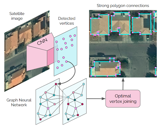
The final model we review, PolyWorld, was published at CVPR 2022 by Zorzi, Bazrafkan, Habenschuss, and Fraundorfer [3]. This model predicts polygons end-to-end and consists of a CNN to extract vertices, a graph neural network to refine the position of these vertices, and an “optimal connection network” to prune, group, and sequence the vertices into polygons.
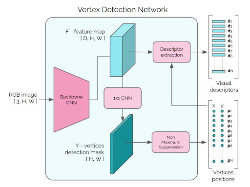
The first part of the model, the vertex detection network, is a fully convolutional network that outputs a feature map and a vertex detection map. The vertex detection map classifies each pixel based on whether or not it contains a vertex. The mask is filtered using non-maximum suppression to find the N peaks with the highest probability. The positions of these peaks are used to select the corresponding feature embeddings from the feature map, which represent a set of candidate vertices.
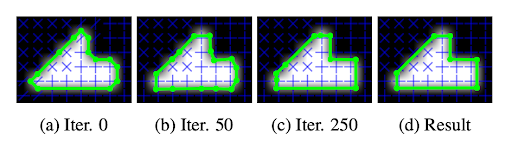
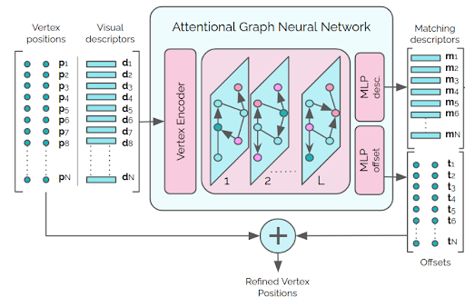
These vertex embeddings and corresponding positions are then passed to an attentional graph network (described below) to aggregate information across the vertices. The input to the graph network is a complete graph (ie. a graph where all nodes are connected to one another) with a node for each vertex. The output of the graph network is a feature vector for each vertex called a “matching descriptor” (the name of which will make more sense later) and a positional offset for each vertex that can be used to refine the predicted position.
The input to a graph network is a graph structure and feature vectors for each node. Each layer updates the feature vector for each node as a function of its neighbors’ feature vectors. With each successive layer, information is propagated through the network via edge relationships. The activation function and associated weights are shared by all nodes. A CNN can be seen as a special case of a graph network where the graph is grid structured. In an attentional graph network, the activation function takes a weighted average of a function of the neighbors. These weights are computed using a self-attention layer which decides how much each node should “attend” to each of its neighbors. Using a complete graph structure, if most of the attention values are negligible, the graph structure is effectively computed dynamically as a function of the input.
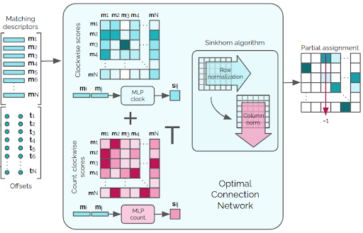
Given the matching descriptors for each vertex, the “optimal connection network” outputs the optimal way of connecting the vertices together into a set of polygons. This network specifies the three components that comprise an optimization system:
- A representation for solutions to the problem
- A function that scores solutions
- A mechanism for finding the solution with the best score
The network represents a set of polygons as an adjacency matrix for a graph with a node for each vertex. Each node is matched with exactly one other node: the next node in a traversal of the polygon, or itself if the node is not part of a polygon. This means that each row and each column should have exactly one entry that is non-zero. A matrix of this form is called a permutation matrix because it permutes the rows of another matrix when it is applied as an operator.
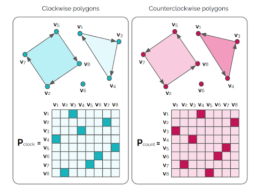
The scoring function for permutation matrices uses a score matrix which contains the affinity between each pair of vertices which is based on the matching descriptors for those vertices. The score for a permutation matrix is then the sum over the element-wise product of the score matrix and the permutation matrix. It turns out that optimizing this scoring function is an instance of the assignment problem, a classic combinatorial optimization problem!
The assignment problem is perhaps best introduced with a concrete example. We are given a set of agents (Paul, Dave, and Chris), and a set of tasks (clean bathroom, sweep floors, and wash windows), and need to assign each agent to a different task. Furthermore, there is a cost matrix, shown below, which contains the cost for each agent to perform each task. The goal is to find the assignment that minimizes the total cost. In this case, the optimal assignment is to have Paul clean the bathroom, Dave sweep the floor, and Chris wash the windows which has a cost of $6.
| Clean Bathroom | Sweep Floors | Wash Windows | |
| Paul | $2 | $3 | $3 |
| Dave | $3 | $2 | $3 |
| Chris | $3 | $3 | $2 |
The optimal matching network solves the same problem except that vertices replace agents and tasks, and the score matrix replaces the cost matrix. In other words, the problem is to match each vertex with one other vertex in a way that minimizes cost. The assignment problem is typically solved using the Hungarian algorithm which runs in time cubic in the number of vertices. However, we cannot simply use the Hungarian algorithm during training since it is not differentiable or GPU efficient. Instead, we use the Sinkhorn algorithm which solves the same problem, but is differentiable and GPU efficient. The algorithm alternates between normalizing rows and columns, and is run for 100 iterations in the PolyWorld paper. Unlike in PolyMapper, there is no need to first detect objects with this method. Instead, vertices are grouped into multiple polygons as a side effect of solving the assignment problem!
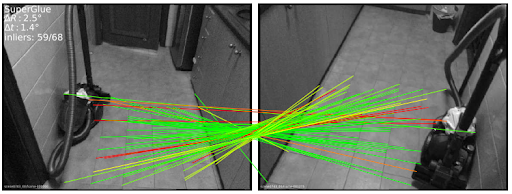
The use of a differentiable version of a classic algorithm as a module within a neural network is a powerful addition to the deep learning toolkit. A similar approach, and a likely inspiration for PolyWorld, was used in a model called SuperGlue. It uses the Sinkhorn algorithm to find an optimal matching between patches located within pairs of related images. These pairs could come from a sequence of image frames in a video, or a binocular camera system. Solving the correspondence problem is a first step in various downstream 3D computer vision tasks such as localization and structure from motion.
Despite having better performance than the frame fields models on the CrowdAI dataset, PolyWold does not have the ability to generate polygons with holes, or handle buildings with shared walls. However, the authors offer some ideas for how the model could be modified to handle these cases. The model and inference (but not the training) source code is open source, but has a restrictive license that only permits its use for research.
Results
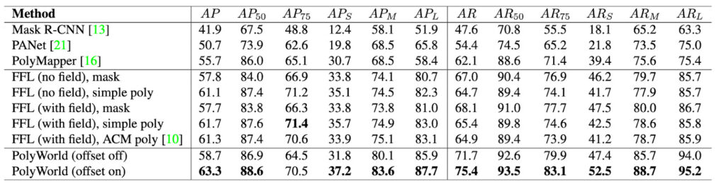
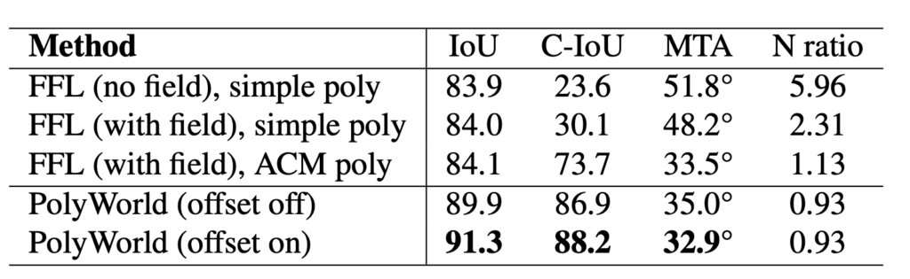
Here, we briefly summarize experimental results from the PolyWorld paper which compares the performance of PolyWorld to instance segmentation baselines, PolyMapper, and Frame Field Learning. The models were evaluated using the test set of CrowdAI using the various metrics described above. Overall, PolyWorld performs better than the other methods on most metrics, and the instance segmentation baselines perform the worst. These results are listed in the tables below.
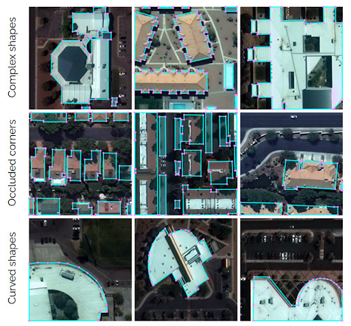
For a more intuitive understanding of how the methods perform, we can look at visualizations of their predictions on different images. Below are examples showing that PolyWorld can handle difficult cases including complex shapes, occluded corners, and curved shapes.
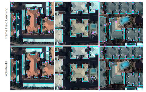
Below is a comparison of PolyWorld and FFL. PolyWorld is apparently better at generating right angles and more parsimonious polygons with fewer vertices.
Conclusion
To help create a map of all the world’s buildings, we can use machine learning to train models that output polygonal building footprints from satellite and aerial imagery. However, training these models requires a large amount of training data, which needs to have very high resolution. Thanks to open datasets such as Ramp, SpaceNet, OpenCities AI, and CrowdAI, researchers can compare the performance of different models, and release those models to the public. Predictions of building footprints can be evaluated using the usual metrics like IoU and AP, but there is a need for new metrics specially designed for this use case. For example, max tangent angle error and complexity-aware IoU are designed to penalize domain-relevant mistakes such as overly complex polygons and rounded corners.
Semantic segmentation and instance segmentation can be used to extract building footprints, but the results are usually too sloppy for cartographic applications. By using end-to-end learning and incorporating domain-specific knowledge into models, researchers have developed a variety of more sophisticated model architectures that perform better. PolyMapper uses an RNN to sequentially connect vertices into polygons. Frame field learning uses a novel representation of contours that can better capture sharp corners, which is important for buildings. Finally, PolyWorld uses a differentiable solver for a combinatorial optimization problem to group vertices into polygons.
Unfortunately, all of these approaches are difficult to implement, with many important details left out in this blog, and either aren’t open source or use restrictive licenses. In addition, many approaches cannot handle shared walls between buildings. Given these limitations, these newer methods may not be worthwhile for use cases such as population density estimation that do not require high fidelity. However, to generate cartographic-quality footprints for databases such as OSM, more sophisticated methods are worth a try.
References
[1] Li, Zuoyue, Jan Dirk Wegner, and Aurélien Lucchi. “Topological map extraction from overhead images.” In Proceedings of the IEEE/CVF International Conference on Computer Vision, pp. 1715-1724. 2019.
[2] Girard, Nicolas, Dmitriy Smirnov, Justin Solomon, and Yuliya Tarabalka. “Polygonal building extraction by frame field learning.” In Proceedings of the IEEE/CVF Conference on Computer Vision and Pattern Recognition, pp. 5891-5900. 2021.
[3] Zorzi, Stefano, Shabab Bazrafkan, Stefan Habenschuss, and Friedrich Fraundorfer. “PolyWorld: Polygonal Building Extraction with Graph Neural Networks in Satellite Images.” In Proceedings of the IEEE/CVF Conference on Computer Vision and Pattern Recognition, pp. 1848-1857. 2022.